HOME
GIFU

This is a tutorial to calculate Gibbs free energy of Water molecule. We will use Thermo_pw package. It is a driver of quantum-ESPRESSO (QE) routines. We can use it for several jobs like convergence tests, phonon frequencies, electronic bands, elastic constants, Quassi-harmonic Approximation (QHA) properties, etc. You can read the description and any required information from Thermo_pw main page.

This tutorial assumes:

1. You already have QE along with Thermo_pw instaled in your system.

2. You already have some basic skills for using QE in linux system.

3. You already have some basic knowledge about QHA and any related physical quantities.

There are two main steps of this tutorial. First, we relax the Water molecule using pw.x to get optimized geometry. Then we use this geometry to calculate the Gibbs free energy using thermo_pw.x.

1 Optimization

I provide a minimum keyword input file for relax calculation using pw.x. You can check pw.x input description to add other preferable keywords.

 
 
 
&CONTROL 
 calculation=’relax’, 
 pseudo_dir=’./’, 
/ 
&SYSTEM 
 ibrav=0, 
 ntyp=2, 
 nat=3, 
 ecutwfc=50, 
/ 
&ELECTRONS 
/ 
&IONS 
/ 
ATOMIC_SPECIES 
O 15.999 O.pbe-n-kjpaw_psl.1.0.0.UPF 
H 1.00784 H.pbe-kjpaw_psl.1.0.0.UPF 
 
ATOMIC_POSITIONS (angstrom) 
O      0.92370.93661.0272 
H      0.64490.52150.1971 
H      1.89160.91580.9856 
 
K_POINTS gamma 
 
CELL_PARAMETERS {angstrom} 
       15.00  0.00  0.00 
       0.00  15.00  0.00 
       0.00   0.00   15.00
 

Explanation of several important keywords are as follows.

calculation=’relax’, This specify our calculation type that is structural optimization.

pseudo_dir=’./’, This specify that the pseudopotential files is in the same directory with the input file.

ibrav=0, This is specify that we do not use any crystal structure, since our system is an isolated molecule.

ntyp=2, nat=3, This specify that our system consist of 2 types of atoms (H and O) with total 3 atoms.

ecutwfc=50, This specify that the kinetic energy cutoff used is 50 Ry. There is a minimum value recommended inside the pseudopotential file of each element. We should make sure that we use higher value than the recommended one. Or, it is better if we optimize this parameter. We can optimize it manually or automatically using Thermo_pw.x (you can found the tutorial here).

O 15.999 O.pbe-n-kjpaw_psl.1.0.0.UPF This specify the symbol of the element, its atomic mass, and its pseudopotential, respectively. They are separated by at least one space. In this tutorial, we use projected augmented wave (PAW) pseudopotentials along with PBE functional. This information can be seen inside the pseudopotentials file.

ATOMIC_POSITIONS (angstrom) Several lines below this card specify the geometry of our system. For visualisation purposes, make sure that every atoms are in positive axes.

CELL_PARAMETERS {angstrom} There lines below this card specify the geometry of our cell, that is a 15 Å $\times$ 15 Å $\times$ 15 Å box. This huge cell will limit the interaction between the periodic systems.

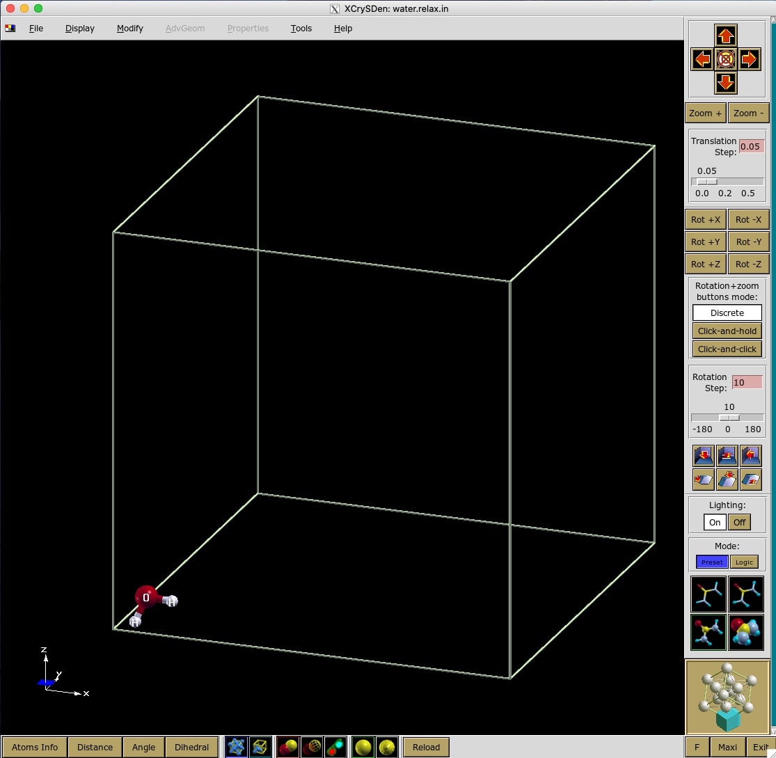
I save the input file as water.relax.in. However, any name and extension is OK. If you done everything right, you should can visualize the input file using XCrySDen program (see Figure 1).

Run the input file using pw.x program:
pw.x < water.relax.in > water.relax.out.

Once the calculation done (denoted by line: JOB DONE.) and the relaxation converged (denoted by line: bfgs converged), we can extract the output geometry of our system. Make sure to take the geometry of the very last cycle of the calculations, that is the one written between Begin final coordinates and End final coordinates, as follows.

 
 
 
Begin final coordinates 
 
ATOMIC_POSITIONS (angstrom) 
O   0.9242104056    0.9361038386    1.0261204507 
H   0.6413561051    0.5206923851    0.1956086279 
H   1.8946334893    0.9171037763    0.9881709214 
End final coordinates
 

We use this coordinates to make the input file for thermo_pw.x which is explained in the next section.

2 Gibbs Free Energy Calculation

We need three input files for this section: an input file for (1) pw.x and (2) ph.x, as well as a file called (3) thermo_control. File (1) will be used for an scf calculation for a fixed geometry obtained from the previous section. The result will be used for phonon calculation using file (2). And finally, file (3) will control the calculation for the Gibbs free energy. The details of each input file are as follows.

2.1 pw.x input file: water.scf_disp.in

 
 
 
&CONTROL 
 calculation=’scf’, 
 prefix=’water’, 
 pseudo_dir=’./’, 
/ 
&SYSTEM 
 ibrav=0, 
 ntyp=2, 
 nat=3, 
 ecutwfc=50, 
/ 
&ELECTRONS 
/ 
&IONS 
/ 
ATOMIC_SPECIES 
O 15.999 O.pbe-n-kjpaw_psl.1.0.0.UPF 
H 1.00784 H.pbe-kjpaw_psl.1.0.0.UPF 
 
ATOMIC_POSITIONS (angstrom) 
O      0.9242104056    0.9361038386    1.0261204507 
H      0.6413561051    0.5206923851    0.1956086279 
H      1.8946334893    0.9171037763    0.9881709214 
 
K_POINTS AUTOMATIC 
1 1 1 0 0 0 
 
CELL_PARAMETERS {angstrom} 
       15.00  0.00  0.00 
       0.00  15.00  0.00 
       0.00   0.00   15.00
 

Most of the keyword is the same with the previous section. The changes are as follows.

calculation=’scf’, This specify the calculation only for a single SCF.

prefix=’water’, This gives identity for the calculation files. These files will be called again in the ph.x calculation.

K_POINTS AUTOMATIC In this calculation we use a thicker k-point, that is $1\times 1\times 1$ with no offset, than in the previous section. This will give a more accurate result, but with more computational cost, for ph.x calculation.

2.2 ph.x input file: ph_control

 
 
 
 &inputph 
  prefix=’water’, 
  fildyn=’water.dyn.xml’, 
  ldisp=.TRUE. 
  nq1=1, nq2=1, nq3=1, 
/
 

Explanation of each keyword are as follows.

prefix=’water’ This should be the same with the one in the pw.x input file.

fildyn=’water.dyn.xml’, This specify the name of dynamical matrix file.

ldisp=.TRUE., nq1=1, nq2=1, nq3=1, This specify the phonon calculation for $1\times 1\times 1$ q-points.

2.3 thermo_control

 
 
 
 &INPUT_THERMO 
  what=’scf_disp’, 
  lgnuplot=.TRUE., 
  find_ibrav=.TRUE., 
  tmin=100, 
  tmax=1000, 
  deltat=100, 
  pressure=1.01325 
 /
 

Explanation of each keyword are as follows.

what=’scf_disp’, This specify the calculation for the harmonic thermodynamic properties: vibrational energy, free energy, entropy, and constant strain heat capacity.

lgnuplot=.TRUE., If you have a gnuplot installed in your computer, then this keyword will trigger the gnuplot to produce a plot for the calculated quantities.

find_ibrav=.TRUE., Since we use ibrav=0, in the pw.x input file, this keyword is needed to build an internal geometry within thermo_pw.x code.

tmin=100, tmax=1000, deltat=100, This specify the minimum, maximum, and interval temperature, respectively.

pressure=1.01325 This specify the external pressure in kbar units. This value is equal to 1 atm.

Once all files are ready, we can perform the calculation using thermo_pw.x:
thermo_pw.x -ni 1 < water.scf_disp.in > water.scf_disp.out.
This calculation is quite heavy so maybe it is necessary to use a parallel calculation, for instance using mpirun.

3 The result

The calculation results is writen in therm_files/output_therm.dat.g1:

 
 
 
# Zero point energy: 0.04113 Ry/cell, 53.99232 kJ/(N mol), 12.90447 kcal/(N mol) 
# Temperature T in K, 
# Total number of states is:         5.89128, 
# Energy and free energy in Ry/cell, 
# Entropy in Ry/cell/K, 
# Heat capacity Cv in Ry/cell/K. 
# Multiply by 13.6057 to have energies in eV/cell etc.. 
# Multiply by 13.6057 x 23060.55 =  313754.7 to have energies in cal/(N mol). 
# Multiply by 13.6057 x 96485.33 = 1312749.8 to have energies in J/(N mol). 
# N is the number of formula units per cell. 
# For instance in silicon N=2. Divide by N to have energies in cal/mol etc. 
#    T              energy             free energy            entropy                Cv 
  0.10000000E+03  0.423834475852E-01  0.384923820814E-01  0.389106550379E-04  0.169694460863E-04 
  0.20000000E+03  0.441451558086E-01  0.339283606134E-01  0.510839759759E-04  0.179624885900E-04 
  0.30000000E+03  0.459593412568E-01  0.284288580445E-01  0.584349440410E-04  0.183336332123E-04 
  0.40000000E+03  0.478196971310E-01  0.223065581204E-01  0.637828475266E-04  0.189163404651E-04 
  0.50000000E+03  0.497489840803E-01  0.157066257241E-01  0.680847167125E-04  0.196894048491E-04 
  0.60000000E+03  0.517599403879E-01  0.871067386213E-02  0.717487775430E-04  0.205364022741E-04 
  0.70000000E+03  0.538572252200E-01  0.137121074625E-02  0.749800206768E-04  0.214133463037E-04 
  0.80000000E+03  0.560433797448E-01 -0.627492940703E-02  0.778978864398E-04  0.223132920112E-04 
  0.90000000E+03  0.583204529630E-01 -0.142004963852E-01  0.805788326091E-04  0.232300298536E-04 
  0.10000000E+04  0.606894948723E-01 -0.223845214090E-01  0.830740162812E-04  0.241499232497E-04
 

Note that the energies written in this file is the correction energies. That means, we need to sum it with the total electronic energy obtain from pw.x calculation to get for instance the total Gibbs free energy of the system. You can get the total electronic energy from water.scf disp.out file in the ! total energy = line.

That’s all. Don’t forget your diner.